Written with <3 by Seth Goldin & Teo Dimov as a free open-access educational resource with insights, edits, and figures from Anthropic’s Claude 3.5 Sonnet and OpenAI’s o1 models.
Special recognition goes to Katherine He, alongside our reviewers and contributors: Tristan Brigham, Rajat Doshi, Grace Gerwe, Gashon Hussein, Linda He, Houjun Liu, Mason Wang, Skylar Wang, and numerous others whose insights shaped this work.
Please report any errors or inaccuracies to teo.i.dimov [at] gmail. April 8, 2025.
Introduction
Before you begin, why read this over the billions of other guides to the foundations of artificial intelligence?
The answer lies in who this was written for. Some friends planned to read technical AI papers without a significant formal foundation. We assembled this content to help bridge that gap efficiently—a few hours’ investment with massive upside in technical understanding. If that resonates, you are in the right place.
This primer won’t teach you everything about machine learning; the field overflows with jargon. You could spend thousands of hours exploring these topics—that’s called a PhD. Instead, this text is intended to enable rapid entry into technical AI discourse, taking you from 0 to 0.5.
There’s a common saying: "learning Chinese is a five-year lesson in humility." The same holds for AI. Mastering every area is improbable. Yet although specialties differ, they share a common language. This text aims to help you become fluent in that shared language.
A Note on AI for Education
We are exceptionally optimistic about the synergies AI brings to education. As such, much of this document was edited and formatted using state-of-the-art large language models. In some cases, AI provided incredible explanations or diagrams for difficult concepts; our work optimizes for clarity and helpfulness over humanness. We are excited that the capabilities of AI as an educational copilot will only improve in the coming years.
1 Defining AI
You’ve noticed we’ve used AI and ML interchangeably. Let’s clarify the difference:
Artificial Intelligence (AI) describes computational systems capable of performing tasks that traditionally required human intelligence. AI can be narrow, designed for specific applications, or general, demonstrating adaptability across various intelligence-demanding functions.
Machine Learning (ML) represents a subset of AI focused on algorithms that identify patterns from data rather than following explicit programming. Within ML, Deep Learning encompasses approaches using multi-layered models to extract increasingly complex patterns from data, often achieving unprecedented performance in specialized tasks.
Fundamentally, artificial intelligence systems undertake domains previously considered uniquely human, such as learning and reasoning. Rather than rigidly programming systems—the traditional paradigm of computer engineering—ML enables adaptive, evolving approaches.
The following chapters will build upon these foundational concepts, addressing the computational aspects of AI/ML systems—data processing and algorithmic approaches - beginning with the essential mathematical concepts in the next section.
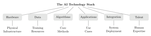
2 Mathematical Foundations
This section covers essential Linear Algebra, Calculus, and Statistics needed to understand AI foundations. It is by no means exhaustive. However, it is background that enables movement beyond abstraction into high-level technical comprehension.
Why does this matter? Many surprisingly simple AI concepts are encoded in the language of mathematics. Linear algebra—the first field of math we cover—provides a framework for converting many of the intuitive, geometric concepts of AI into more versatile algebraic (numerical) forms. Calculus then lets us work with these numerical representations to achieve powerful results such as the "learning" that powers AI. And statistics is central to understanding data distributions, making predictions under uncertainty, estimating model parameters, and evaluating model performance.
2.1 Mathematical Notation
What follows is essential notation for ML foundations. This section serves as a reference index rather than material to master on first reading.
Sets and Spaces
| natural numbers | |
| integers | |
| real numbers | |
| -dimensional vector space |
Logic and Operations
| "for all" | |
| "there exists" | |
| "is an element of" | |
| "is a subset of" | |
| "implies" |
Variable Conventions
| indices | |
| dimensions, sizes | |
| input/output variables | |
| weights | |
| bias terms | |
| parameters (general) | |
| learning rate | |
| regularization parameter |
Vectors and Matrices
| vectors (bold lowercase) | |
| matrices (bold uppercase) | |
| -th element of vector | |
| element at position | |
| transpose of | |
| inverse of matrix | |
| norm of vector |
Set Operations
ML-Specific Notation
| loss function | |
| objective/cost function | |
| predicted output | |
| dataset | |
| input feature matrix | |
| target/output matrix |
Asymptotic Analysis
is if there exist constants and such that:
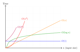
| Complexity Class | Time |
|---|---|
| Constant | |
| Logarithmic | |
| Linear | |
| Quadratic | |
| Exponential |
2.2 Linear Algebra
Linear algebra forms much of the backbone of machine learning. Let’s explore some key concepts.
2.2.1 Matrices and Matrix Operations
A matrix is fundamentally a list of numbers with dimensions , where represents rows and represents columns. A vector is a 1D matrix, while a tensor extends this to higher dimensions with additional metadata for AI operations.
Matrix Addition
Subtraction (which is effectively just addition of a negative number) works similarly. Both match elements together in same-shape matrices and perform the operation one-by-one.
Matrix multiplication, on the other hand, comes in several forms:
Types of Matrix Multiplication
Scalar multiplication: Multiply every element by a scalar
Hadamard product : Element-wise multiplication
Dot product: For vectors, multiply corresponding elements and sum
Matrix multiplication: Each element is the dot product of a row and a column
Kronecker product : Block-wise multiplication
Note that if is and is , then is .
Example 1: 3×3 Matrix Multiplication
Example 2: 3D Matrix Multiplication
Matrix and (2×2×2 tensors):
Batch multiplication (element-wise matrix multiplication):
Note that for matrix multiplication, the number of columns in the first matrix must be equal to the number of rows in the second ( = ). This will result in dimensions in the format ( × ), where the number of rows in the first matrix are equal to the number of columns in the second matrix.
2.2.2 Determinants
The determinant serves as a matrix’s "fingerprint", revealing important properties:
The Determinant
2×2 matrices:
3×3 matrices (Sarrus’ rule):
Determinants describe significant information about a matrix, such as whether it can be inverted, as well as information about each of the individual vectors.
A column of a matrix is considered linearly independent if it cannot be composed by somehow combining (through scaling and adding) the other columns. In a geometric context, the determinant also describes how much a matrix scales a shape.
Linear Dependence and Zero Determinant
A set of vectors is said to be linearly dependent if there exist scalars , not all zero, such that This implies that at least one vector can be written as a linear combination of the others.
Example: Consider the matrix Its rows are and . Notice that which shows that is a linear combination of ; hence, the rows of are linearly dependent. This is confirmed by the determinant:
In machine learning, we typically care that our determinant is nonzero (so that we can perform a versatile set of operations on our matrix). Additionally, the determinant of a matrix is invariant, or unchanged, by many of the operations that you perform on matrices. These include elementary row operations, where you essentially take linear combinations of rows, and transposition, which involves swapping a matrix’s rows with its columns. This invariance provides us with valuable information as you operate across large amounts of matrices.
Transposing a Matrix
Given some matrix A:
The transpose of is expressed as:
2.2.3 Vector Spaces
A vector space represents concepts as points in multi-dimensional space, where mathematical operations correspond to meaningful transformations. Perhaps the most intuitive three-dimensional vector space is , where you measure distance between points by taking the Euclidean Distance between them:
Euclidean Distance
Given 3D points , you compute their euclidean distance as:
To get you more familiar with notation, this can be more compactly expressed as:
In addition to our notion of Euclidean distance, similarity between data points can be measured using various distance metrics. A common one is cosine similarity, which measures the angle between the vectors, producing values from -1 (opposite) to 1 (identical), independent of the magnitude of the vector. This metric effectively captures semantic similarity by evaluating how closely vectors point in the same direction.
Cosine Similarity is dot product and , are vector magnitudes.
The key idea here is that gets closer to 1 for similar vectors. Hence, a larger cosine similarity means vectors are similar (unlike the Euclidean metric, where smaller distances represent closeness).
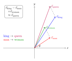
Word embeddings like Word2Vec and GloVe leverage this property by mapping words to vectors such that semantic relationships become mathematical operations. The canonical example above demonstrates this elegantly.
This allows us to perform robust mathematics and searching in our embedding space. These properties of embeddings are what allow us to search for "similar" words or phrases, even when exact matches don’t exist.
2.2.4 Eigenvectors and Eigenvalues
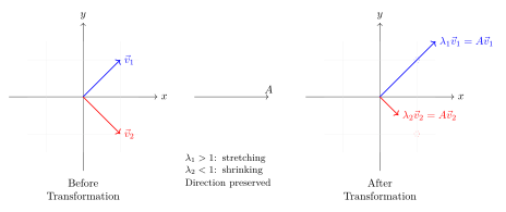
Eigenvectors represent fundamental directions where transformation results only in scaling. The scaling factor is the corresponding eigenvalue (). The eigenvalue equation is .
Finding Eigenvectors and Eigenvalues:
1. Set up
2. Solve for eigenvalues
3. Find corresponding eigenvectors (solve for )
4. Normalize if needed
2.2.5 Matrix Convolution
Matrix convolution represents a specialized operation where a kernel (or filter) matrix slides across an input matrix, computing dot products at each position.
Convolution "Flip and Slide" Process:
1. Flip kernel horizontally and vertically
2. Align with input matrix section
3. Compute dot product
4. Store result in output matrix
Example: 1D Convolution
Convolution is a more powerful tool than simple multiplication to detect patterns in data. As such, convolution powers many image processing tasks, such as Convolutional Neural Networks (CNNs).
To preserve input dimensions, we can use zero padding: surrounding the input matrix with zeros. This enables full convolutions across the entire input space.
You can also adjust the stride, which is the step size the convolutional filter uses as it moves across the input data. A stride of 1 moves the filter one pixel at a time, while a stride of 2 moves two at a time, skipping every other pixel. Larger strides mean less overlap between receptive fields (RF), the region in the input space that affects some particular neuron, and result in smaller output feature maps. More on this in section 5.
Example: 2D Convolution with Padding
Input matrix and kernel :
Flip horizontally and vertically:
Slide and compute the full 3×3 output (stride = 1):
Final result:
2.3 Calculus
This primer is not going to teach you Calculus—that’s what 3Blue1Brown is for. However, a few concepts are critical for ML and this section will briefly review them. There is some assumed knowledge here: for example, you should already know what a derivative is (rate of change), and how to find one.
2.3.1 Gradient Descent
Gradient descent is an optimization technique that attempts to minimize "loss", where loss represents the error in an algorithm. The gradient is the slope of the function—a vector of partial derivatives with respect to its inputs. In 2D, it’s simply the slope; in higher dimensions, it points in the direction of steepest increase.
As such, if you have some n-dimensional surface, on which you are trying to find some local extrema (minimum or maximum), then you can use the gradient as a sort of compass at every point to guide us in the right direction.
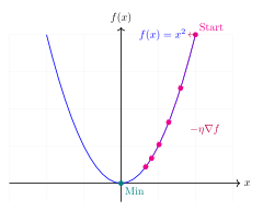
Gradient Descent Process:
1. Randomly initialize weights
2. Calculate gradient at current position
3. Scale gradient by learning rate ()
4. Move in direction of negative gradient
5. Repeat until convergence or maximum iterations reached
There are three popular variants for actually implementing these updates. Batch Gradient Descent (BGD) uses all the data for each update, while Stochastic Gradient Descent (SGD) and Mini-batch Gradient Descent use a single sample and a small batch of samples, respectively.
Although Batch Gradient Descent perfectly computes the optimal, steepest direction at every update point, it takes a long time since it uses all of the data. Stochastic and minibatch GD, on the other hand, compute an approximate optimal direction and do it much more efficiently due to their lower data requirement. The resulting gradient estimate is an unbiased estimator of the true gradient for a given set of function parameters. As such, they are often used in practice in place of BGD.
The learning rate is important: too small means slow convergence (you have to take too many steps to get anywhere on your function), too large risks overshooting (you completely miss your optimum by moving the parameters too far). Consider also local versus global minima: in a hilly landscape, local minima represent small valleys while the global minimum is the lowest point overall.
Gradient Ascent, the sister algorithm, maximizes reward values by adding rather than subtracting the scaled gradient. While descent minimizes loss in neural networks, ascent commonly maximizes rewards in reinforcement learning.
This leads us to the two most important math concepts for understanding machine learning: partial derivatives and the chain rule. We’ve addressed them briefly here, and we recommend you go through some other resources until these feel intuitive. They are the backbone behind all the magic in the chapters to come.
2.3.2 Partial Derivatives
Partial derivatives are important for functions of multiple variables—virtually everything in ML. They measure how a function changes when adjusting one variable while keeping others constant; in other words, how each variable changes with respect to the other variables. As such, they allow us to determine how changing one specific parameter changes the entire multivariate function. This is best shown through an example:
For :
(treat y as constant)
(treat x as constant)
In neural networks, we need partial derivatives because loss functions depend on thousands or millions of parameters simultaneously. These partial derivatives tell us exactly how to adjust each weight to minimize the loss function.
The gradient vector, composed of all partial derivatives, points in the direction of steepest increase—meaning if we moved in that direction, our loss would get worse fastest. So we move in the opposite direction during training, which is the direction where our loss will decrease most rapidly.
2.3.3 Chain Rule
The chain rule is critical for training neural networks through backpropagation, a concept we’ll explain later on. Essentially, the chain rule is a mechanism for answering the question of "how does changing some variable x affect variable y?".
The answer lies in combining – or "chaining" together – partial derivatives. This lets us track how the change flows through each variable into our final desired relationship. For example:
If , then:
This finds how each parameter affects the final output, making gradient-based learning possible. Without the chain rule, we couldn’t efficiently compute gradients in deep networks with many layers. For example, if we have , we can set and , giving us .
These concepts form much of the mathematical foundation of neural network learning: forward pass computes predictions, partial derivatives compute gradients, chain rule propagates gradients backward, and gradient descent updates weights.
2.4 Probability and Statistics
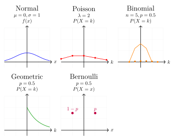
Probability distributions help estimate the likelihood of outcomes. Although hundreds exist, a few distributions form the foundation of ML. The golden rule: Probabilities always sum to 1.
2.4.1 Essential Distributions
Bernoulli/Uniform Distribution
Two discrete outcomes, like heads/tails. Fair die rolls give a uniform distribution (1/6 each).
Binomial Distribution
The Binomial Distribution requires n distinct trials, binary success/failure, a constant probability p, independent trials, and the counting of total successes.
Poisson Distribution
The Poisson distribution models random events at fixed rate . It assumes independent time intervals, uniform distribution across equal intervals, that probability scales with time, and that there are no simultaneous events as intervals shrink.
Geometric Distribution
"Failures before success" with probability p. Negative binomial extends this to r successes.
Normal/Gaussian Distribution
The infamous Normal distribution is a perfect bell curve. By Central Limit Theorem, sums of independent samples approach a normal distribution (i.e. the more things you sum, the more “normal” their distribution becomes).
2.4.2 Bayes’ Theorem
Bayes’ theorem tells us the probability of an event occurring given that you have observed another related event.
Bayes’ Theorem where:
: Posterior probability (A given B)
: Likelihood (probability of B given A)
: Prior probability (probability of A)
: Evidence (probability of B)
The posterior probability P(A|B) represents what you believe after seeing the evidence. The likelihood P(B|A) shows how probable our evidence is if our hypothesis is true. The prior probability P(A) reflects our initial beliefs or assumptions. Finally, P(B) represents the overall probability of observing our evidence and is a normalizing factor to keep our probabilities coherent.
Consider predicting snowfall in the city of New Haven: With a 30% prior probability of snow P(A) and a 70% probability of clouds when it is snowing P(B|A), given an overall 50% probability of clouds P(B), Bayes’ theorem updates our belief to a 42% probability of snow given that we observe clouds P(A|B).
This concludes our section on fundamental mathematics. We’ve included several more notes in our appendix section, which you can find at the end of the primer. There is much you could go deeper into here, and should. In the next section, we will review the core ML concepts that build on these topics.
3 ML Foundations
Before diving into specific algorithms and architectures, it is helpful to understand some fundamental principles regarding how we develop models, and that govern how models learn and generalize.
At its core, machine learning works because the patterns that exist in the real world—which are expressed in large dimensions—can be adequately reduced to representations in lower dimensions.
For example, a human face can be explained with millions of pixels, yet we can capture its most important features with just a few hundred variables that encode characteristics like face shape, eye position, and expression. This concept is known as the "manifold hypothesis"; this reduction is the reason models are good at taking in enormous amounts of information and learning sensible patterns.
3.1 Bias-variance tradeoff
The bias-variance tradeoff is one of the fundamental challenges in machine learning, describing the tension between two types of error that occur in machine learning models.
Bias reflects the error introduced by approximating a real-world problem with a simplified model. It measures how far off our model’s predictions are from the true (correct) values, even with an infinite amount of training data. High bias leads to underfitting, where the model makes oversimplified assumptions about the underlying patterns in the data.
Variance, conversely, measures how much our model’s predictions would fluctuate if trained on different datasets. High variance leads to overfitting, where the model becomes too sensitive to the noise in the training data rather than learning the true underlying patterns. The total error of a model can be decomposed into three parts: where irreducible error represents the noise inherent in the problem that no model can eliminate.
The tradeoff emerges because these components are inversely related: as you decrease one, you typically increase the other. Simple models tend to have high bias but low variance, making consistent but potentially oversimplified predictions. Complex models are the opposite, capturing subtle patterns but risking learning noise. Finding the sweet spot between these extremes often determines the success of a machine learning model.
3.2 Cross-validation
Cross-validation ensures models are developed in a way that properly manages the bias-variance tradeoff, and helps us understand how our model will perform on data it hasn’t seen before. The main idea behind cross-validation is simple: divide your dataset into multiple parts and use different portions for training and testing. This process provides a more robust estimate of model performance than a single train-test split.
There are several common approaches for implementing cross-validation:
Holdout Validation is the simplest method, where data is divided into training and test sets, typically with 50-80% allocated for training and the remainder for testing. Although straightforward to implement, this approach can be wasteful of data and may provide unstable estimates if the split happens to be unrepresentative.
K-fold Cross-validation is a more sophisticated solution dividing data into k equal segments, often 5 or 10. The model trains k times, using a different fold as the test set each iteration, while the remaining folds serve as training data. The results are averaged across all iterations, giving a mean performance metric and its variance. This approach can be especially valuable when working with limited data.
Leave-one-out Cross-validation (LOOCV) takes this concept to its logical extreme. The model trains on all but one data point and tests on the "held-out" point, repeating for the whole dataset. While this provides nearly unbiased estimates of model performance, it is computationally expensive with large datasets.
Stratified Cross-validation has each fold maintain the same distribution of target variables. This is helpful when dealing with imbalanced datasets, where some outcomes are much rarer than others. For instance, in a disease detection model where positive cases are uncommon, stratification guarantees that each fold contains a representative proportion of positive cases.
3.3 Regularization
Regularization helps defend against overfitting in machine learning models. It works by adding penalties to the model’s loss function that discourage unnecessary complexity. The two most common forms are L1 (Lasso) and L2 (Ridge) regularization. Each adds a different type of penalty term to the loss function:
where controls regularization strength and represents model weights
L1 regularization tends to produce sparse solutions by forcing some weights to exactly zero, effectively performing feature selection. L2 regularization keeps all features but shrinks their importance uniformly, preventing any single feature from dominating the model.
The Elastic Net combines both approaches:
Modern deep learning introduces additional regularization techniques like dropout (randomly deactivating neurons during training) and early stopping (halting training before overfitting occurs).
3.4 Feature Engineering
Feature engineering transforms raw data into formats that machine learning models can better utilize. While a dataset might contain valuable information, how that information is represented often matters as much as the information itself.
A feature transformation is a term encompassing a number of approaches. Temporal transformations focus on converting timestamps into more meaningful representations, such as cyclical features and extracting time-based patterns like weekday/weekend distinctions or seasonal variations. Numerical transformations involve techniques like scaling and normalization, applying log transformations to handle skewed data, and binning continuous variables into discrete categories when appropriate.
Categorical transformations play an equally important role, employing methods such as one-hot encoding, label encoding, and feature hashing to convert categorical data into formats that models can process effectively. Interaction features add another layer of sophistication by combining multiple features, creating meaningful ratios, and generating polynomial features to capture more complex relationships in the data.
External data enrichment provides another powerful avenue for feature enhancement. This might involve incorporating data from public datasets, APIs, or other external sources to provide additional context to your model. The idea is to add new features relevant to your core problem while avoiding unnecessary complexity.
3.5 Curse of Dimensionality
The curse of dimensionality refers to the challenges that arise when working with high-dimensional data. As the number of dimensions increases, the volume of the space increases so rapidly that available data becomes sparse.
This phenomenon has several important consequences. Data sparsity increases exponentially with dimensions. Distance metrics become less meaningful. Required sample size grows exponentially. And computational complexity increases significantly.
To combat these challenges, we can use dimensionality reduction techniques like PCA (Principal Component Analysis) or t-SNE (t-Distributed Stochastic Neighbor Embedding) before training our models.
3.6 Natural Language Processing
Natural Language Processing (NLP) interprets and predicts text data. The fundamental unit is the token, created through tokenization which breaks text into smaller units. While word-level splitting might seem intuitive, language complexities necessitate sophisticated approaches.
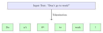
Tokenization challenges include handling contractions (e.g., "don’t" → "do" + "n’t"), managing punctuation and special characters, and processing URLs and special cases.
Modern approaches favor subword tokenization, balancing word and character-level analysis. Training data comprises vast collections of human-written text from web scrapes, Wikipedia, books, and various sources. These sequences undergo embedding into vector spaces for processing. Each token in the result is typically represented by a vector for modern machine learning models like language models.
These concepts, from cross-validation to regularization, form the backbone of machine learning. Understanding them deeply helps practitioners make effective decisions about model development and deployment.
4 Classical ML Algorithms
Machine learning algorithms can be divided into three main categories: supervised, unsupervised, and reinforcement learning. Supervised learning works with labeled data to predict specific outcomes, whereas unsupervised learning operates on unlabeled data to discover inherent patterns. Reinforcement learning differs from both, learning through interaction with an environment and receiving feedback (rewards or penalties).
Supervised learning can be thought of as having a teacher giving out the answers, unsupervised learning must discover the answers, and reinforcement learning learns through trial and error. The following algorithms, though simpler than modern neural networks, remain incredibly powerful.
4.1 Supervised Learning
4.1.1 Linear and Logistic Regression
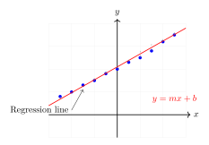
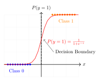
Linear regression is the most straightforward form of supervised learning. The algorithm fits a line through data points by minimizing the distance between each point and its corresponding position on the line. This reveals relationships between variables and predicts outcomes, though note that significant outliers can substantially impact the model’s performance.
The formula is where is the slope (rate of change) and is the y-intercept. Logistic regression follows a similar process but fits data to a sigmoid function instead of a straight line.
4.1.2 Support Vector Machines
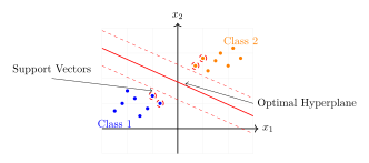
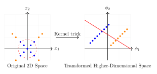
Support Vector Machines (SVMs) excel at finding optimal boundaries, called hyperplanes, between distinct classes in your dataset. Their power lies in the "kernel trick", which projects data into higher dimensions where linear separation becomes possible, without computing the higher-dimensional coordinates. However, this can be costly, typically scaling quadratically with dataset size.
4.1.3 Decision Trees
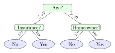
A decision tree is a branching structure where each node represents a decision point testing a specific feature. The tree splits into multiple paths based on these decisions, eventually reaching leaf nodes that provide predictions. Their strength is interpretability; you can trace how the model came to its conclusion.
4.1.4 Random Forests
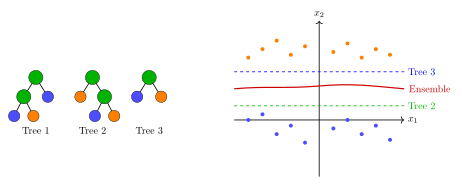
Random Forests address the overfitting tendencies of individual decision trees through ensemble learning. By creating multiple trees trained on random subsets of data, then aggregating their predictions, Forests achieve more robust and generalizable performance—valuable in scenarios with limited data availability.
4.1.5 Gradient Boosting
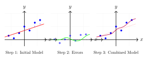
While Random Forests build trees in parallel, Gradient Boosting constructs them sequentially. Each new tree focuses on correcting the errors of its predecessors.
The process involves two critical hyperparameters:
1. Learning rate, which controls the contribution weight of each new tree
2. Number of boosting rounds, which determines the total number of sequential models
This technique particularly shines in scenarios where the data relationships are complex but deep learning would be excessive.
4.2 Unsupervised Learning
4.2.1 Clustering
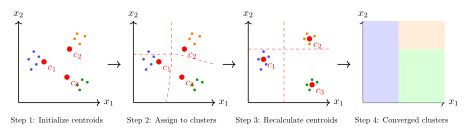
Clustering represents a fundamental approach to discovering natural groupings within data. One widely used clustering algorithm, K-means, follows an elegantly simple process:
Kmeans:
1. Initialize K random centroids
2. Assign each datapoint to its nearest centroid
3. Recalculate centroids as the mean of their assigned points
4. Repeat steps 2-3 until convergence or reaching maximum iterations
An enhanced version, K-means++, improves initialization by strategically selecting starting centroids from the dataset, often leading to better final results. Hierarchical clustering offers another approach, organizing data into a tree-like structure of nested clusters. This method has two variants: Agglomerative (bottom-up), which starts with individual points and merges similar clusters, and Divisive (top-down), which begins with one cluster and divides recursively.
4.2.2 Dimensionality Reduction
Principal Component Analysis (PCA) is a primary dimensionality reduction technique. At its heart, PCA searches for the most informative angles from which to view your data by finding directions (principal components) along which data varies most significantly. Imagine viewing a shadow cast by a complex 3D object—PCA finds the most informative angle, preserving key features while simplifying the representation.
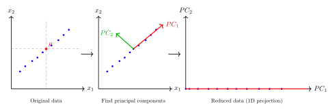
Consider analyzing thousands of face images. Each image has millions of pixels (dimensions), but PCA reveals the most meaningful variation can be captured by a few hundred components—perhaps corresponding to features like face shape or eye position.
Example: Computing PCA
Consider three vectors:
[2 1], [4 3], [6 5]
1. Center data by subtracting mean vector [4 3]:
[-2 -2], [0 0], [2 2]
2. Compute covariance matrix:
[4 4; 4 4]
3. Find eigenvalues:
,
4. First principal direction:
5. Data points projected onto the 1st principal component direction:
This reduces the data to a single dimension without loss of information.
In real-world applications, each direction typically accounts for some proportion of overall variance. Practitioners must balance model simplicity (fewer dimensions) against preserving variance (retaining original information). PCA has limitations, primarily its linear nature—it assumes meaningful patterns can be captured by straight lines and flat planes.
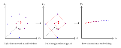
For complex, nonlinear patterns, you can turn to more sophisticated techniques. t-SNE (t-Distributed Stochastic Neighbor Embedding) excels at preserving local structure, making it particularly effective at revealing clusters and patterns that PCA might miss.
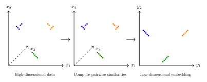
UMAP (Uniform Manifold Approximation and Projection) offers similar capabilities to t-SNE but with better preservation of global structure and significantly faster computation time. It’s particularly valuable for large-scale datasets where both efficiency and accuracy matter.
Each technique serves different purposes: PCA is great for interpretable components and variance preservation, t-SNE excels at visualization and local patterns, and UMAP balances these approaches while scaling effectively. In practice, dimensionality reduction often serves as a crucial pre-processing step in machine learning pipelines, helping reduce noise, speed up computation, and make patterns more visible to both humans and algorithms.
Together, these supervised and unsupervised techniques are foundational parts of the ML ecosystem that you may return to or reference.
4.3 Reinforcement Learning
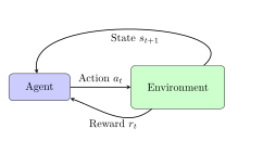
Reinforcement Learning (RL) is about teaching AI to make sequential decisions. RL deals with an agent, essentially an AI-powered decision maker. This agent operates in an environment, where at each state, the agent takes an action which moves it to the next state.
Throughout this process of navigating an environment, the agent experiences feedback, which is a positive reward when the agent does what we want and a negative penalty when it doesn’t.
Many RL problems are formalized as Markov Decision Processes (MDPs), which means that the next state depends only on the current state and action, not on the history of previous states. However, not all RL algorithms are limited to the Markovian assumption, as some consider sequences of past states and actions.
There are two main approaches to solving RL problems. Value-based methods attempt to learn how "good" different states or actions are by estimating their future rewards. Policy-based methods, by contrast, directly learn a mapping from states to actions, typically by learning which actions are most likely to succeed in different situations.
Of course, if these policies are not carefully designed, agents might find undesirable ways to obtain a reward, a phenomenon known as reward hacking. The process of converting qualitative goals into quantitative policy functions is known as the specification problem.
Another big challenge in RL is exploration versus exploitation, which is similar conceptually to how we used these terms when describing optimization.
Exploitation means taking actions known to yield high rewards based on current knowledge, while exploration involves trying new actions on the chance that it results in discovering better strategies. Balancing these competing needs is important for effective learning.
Deep reinforcement learning methods have been the workhorse behind many recent breakthroughs, such as mastering Go and building autonomous robots. The resurgence of the technique also brought about Reinforcement Learning from Human Feedback (RLHF), where models are fine-tuned using human preferences as rewards. RLHF is the reason large language models like GPT output results that satisfy user queries as well as do—they’re literally optimized based on millions of human interactions.
4.3.1 Q-Learning
With Q-learning, the RL agent maintains a "Q-table"—essentially a lookup table that stores the expected reward for each possible action in each possible state. "Q" just refers to the quality of an action in a given state.
When the agent takes an action and receives feedback, it updates its Q-table using:
where is the learning rate, is the discount factor, is the immediate reward, is the current state, is the action taken, and is the next state.
Essentially, we update the old estimate by adding a portion of the difference between the old estimate and the new improved estimate. The new estimate combines the immediate reward and maximum expected (optimal) future reward.
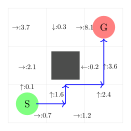
Example: Q-learning in a 3x3 Grid Environment
Consider a 3×3 grid where an agent must navigate from start (S) to goal (G):
1. Initially, the agent has no clue which actions are good (all Q-values are zero)
2. Through exploration, it attempts different paths and receives rewards
3. After many iterations, the agent builds a map of values for every action in each position
4. Eventually, the highest value actions trace the optimal path from start to goal
e.g., at position [1,1], moving right becomes strongly preferred over moving down because the rightward path leads more efficiently to the goal.
4.3.2 Actor-Critic Methods
Actor-Critic methods combine ideal aspects of value-based methods (like Q-learning) and policy-based approaches. As the name suggests, these methods use two primary components:
1. The Critic evaluates actions by learning a value function (like with Q-learning)
2. The Actor determines which actions to take by learning a policy:
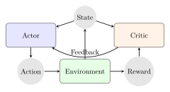
The critic evaluates the actor’s decisions, providing feedback on how "good" or "bad" any given action was. Using such feedback, the actor can continuously improve its policy.
Modern RL systems often implement these algorithms using neural networks instead of tables, allowing them to handle complex environments with vast state spaces, such as robotics and autonomous vehicles.
5 Neural Networks
Neural networks were initially inspired by the structure of neurons (nerve cells) in the human brain. While the function of each individual neuron is quite limited, the emergent complexity that comes from combining millions and billions of neurons is remarkable, allowing us to run prediction, classification, or generation tasks.
We’ll start small with the perceptron, one of the most basic building blocks of neural networks.
5.1 Feedforward Neural Networks
5.1.1 Perceptrons
Put simply, Perceptrons implement a linear decision boundary that separates data points into binary classes. Given some starting weights and biases, they iteratively update their weights by minimizing prediction errors to produce an output for any given input.
Mathematically, perceptrons perform a weighted sum of inputs followed by an activation function. More simply, they are a series of matrix multiplications with a non-linearity applied to the output.
The learning rate controls how quickly weights are adjusted. The algorithm converges when the perceptron correctly classifies all training examples or reaches an acceptable error threshold.
Perceptron Algorithm:
Initialize weights and bias randomly
For each training example:
Calculate predicted output:
Compute error:
Update weights:
Update bias:
Repeat until error is minimized or maximum iterations reached
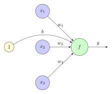
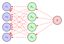
In the above diagram, the perceptron computes the activation function to find . This weighted sum reflects the linear combination of input features, which is passed through an activation function (which we’ll describe in more detail later) to determine whether the neuron fires or not (the output y). The weights and bias are parameters that the network learns during training.
A multi-layer perceptron, or MLP, consists of multiple layers of interconnected neurons. Unlike a single perceptron, however, MLPs allow the network as a whole to learn and represent complex, nonlinear relationships in data.
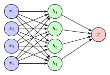
The above MLP showcases an input layer, a hidden layer, and an output layer. Each connection represents the passing of information through non-linear transformations across layers, enabling the network to learn complex patterns.
5.1.2 Activation Functions
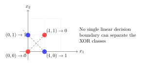
Perceptrons are powerful, but they come with a large limitation: since they are themselves linear functions, combining several of them still yields a linear function. This is best demonstrated through the famous "XOR (exclusive or)" example, where we cannot split the data with a linear decision boundary.
As such, we need a tool that introduces nonlinearities into the mix, such that decision boundaries can take on complex curved shapes (instead of simply being lines).
Enter Activation functions: nonlinearities that enable a neural network to learn more complex transformations. A deep network of purely linear layers collapses into a single linear transformation, making it impossible to learn complex patterns or relationships in data. One of the most commonly used activation functions is ReLU, or Rectified Linear Unit. ReLU retains the value if positive and converts a given input to 0 if negative. It can be written as .
Activation functions help to address the vanishing gradient problem, where gradients become extremely small as they flow backward through deep networks, rendering learning in earlier layers ineffective. With ReLU, the gradient stays 1 for positive values, enabling sparse activation where many neurons output 0. This reduces superposition, when neurons represent multiple concepts. Sparsity is similar to biology, where neurons have threshold activation.
Other common activation functions include Sigmoid, which maps values to the Sigmoid function and outputs between 0 and 1, which is ideal for binary classification.
Another, Tanh (the hyperbolic tangent), outputs between -1 and 1 when zero-centered outputs are ideal, such as with time series or signal processing.
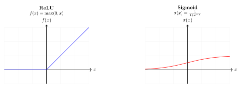
In the above graphs, the ReLU function returns , while Sigmoid outputs values between 0 and 1 using . In short, ReLU makes networks more expressive than a purely linear model, whereas Sigmoid functionally transforms any real-valued number into a probability-like output.
Modern models have introduced variants of these functions. The GELU (Gaussian Error Linear Unit) incorporates probabilistic element into the ReLU, while the SwiGLU introduces gating mechanisms for information flow control (we discuss gates later the GRU section).
5.1.3 Backpropagation
Backpropagation is a mechanism that enables neural networks to “learn” by updating their weights to reduce errors. During the training process, a model is given some input and tasked with making some prediction about it, be it classification or regression. This output is compared with the ground truth, or the output we actually know to be correct (e.g., an image is actually a hot dog). This is known as the forward pass.
The network calculates the error between prediction and truth, then updates its weights based on their contribution to incorrect probabilities. This process propagates backward through layers, with each neuron receiving updates based on its contribution to the final error. Through iteration across the training corpus, the model gradually improves its predictions. After comparing its output to the ground truth, the model then propagates that information backwards through the network (hence backpropagation). In order to do this effectively, the network first computes how much each neuron contributed to the error in the final prediction.
For example, say we’re predicting the probability of an image being a certain number. Suppose the model makes the following prediction, with each entry representing the probability of the image being the corresponding digit index (i.e. 0.01 probability the digit is 0, 0.05 probability the digit is 1, 0.04 probability the digit is 2, etc). This can be encoded in the following vector:
[0.01, 0.05, 0.4, 0.1, 0.15, 0.08, 0.02, 0.12, 0.05, 0.02]
Suppose the digit is actually a 2, that as the ground truth is represented as: [0, 0, 1, 0, 0, 0, 0, 0, 0, 0]
Backpropagation begins by calculating the error, or difference between prediction and truth, for each neuron. Each weight is then updated based on how much it contributed to these incorrect probabilities, strengthening connections that would push the "2" output higher and weakening those activating other digits.
This same process is then applied to the previous layer, using the final layer as the new “ground truth”. Weights that properly predicted values in the final layer are pushed up, and those that did not are pushed down. When this process is applied recursively, every neuron receives a weight update. By iteratively applying this process across a large training corpus, and having the network “learn” from each labeled example, the model improves its predictions to better resemble what it has seen during training.
5.2 Convolutional Neural Networks (CNNs)
5.2.1 Convolutions
As established earlier, a convolution is another type of operation that can be performed on matrices. A convolutional layer uses learned filters to detect patterns in the input, such as textures, edges, or more complex features depending on layer depth. They are frequently used in computer vision tasks that involve images. These filters slide across an image spatially using small windows.
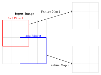
In the preceding diagram, two 3×3 filter windows (red and blue) slide over a 5×5 input image to produce two feature maps. Each filter detects different patterns, creating separate feature maps that represent detected features in the original input.
5.2.2 Pooling Layers
Pooling layers are a type of nonlinearity that allow for dimensionality reduction in image-intensive tasks. There are two main types of pooling layers, mean pool and max pool, and they do basically exactly what you’d expect. Mean/average pooling layers find the average over a section of a matrix and that value represents that section. Max pooling layers find and use the maximum value. Both reduce the spatial dimensions of the data which help reduce computation, provide some spatial invariance (slight shifts in features don’t matter—an object can be detected anywhere in an image), and prevent overfitting. They are commonly used to simplify data for edge detection and image recognition tasks.
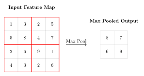
To compute max-pooling, divide a matrix into small non-overlapping squares and then take a window (such as 2x2) and retain only the maximum value. Mean-pooling is a similar process but rather takes the average of the values in that section.
Max pooling layers are typically placed after convolutional layers in a CNN for multiple successive convolutional and pooling layers, allowing the network to learn a hierarchy of features.
5.2.3 Modern Architectures
As neural networks became deeper, researchers encountered a paradox: sometimes adding more layers made performance worse, even though a deeper network should theoretically be able to learn everything a shallower network could. Researchers began experimenting with novel architectures that could more effectively pass information in ever increasingly deep networks.
One such breakthrough came with Residual Networks, commonly referred to as ResNet. The architecture introduced "skip connections”, or shortcuts, in the neural network that allow information to bypass layers. Instead of learning the full transformation across each layer, these networks learn the residual, or the difference between the input and desired output. As such, the final model utilizes only layers that are overall helpful to model performance—and skips those that are not.
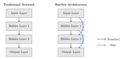
The preceding diagram displays how traditional networks connect layers sequentially, while ResNets add skip connections (blue) that bypass layers, helping overcome the vanishing gradient problem during training and enabling the training of deeper networks.
This design was further enhanced through DenseNet, an architecture featuring connections from each layer to every other layer in a feed-forward fashion. Residual connections have outlived their origins with simple CNNs, and have largely become standard in many modern deep learning implementations.
5.2.4 Softmax
Ultimately, classification networks output class likelihood, which is represented internally as probabilities for each class. To do this, we need a mechanism for converting raw final scores, such as -2.4, 0.5, and 1.7, into associated probabilities (that sum to one). So, we employ the softmax mechanism, which simply maps these raw scores to probabilities as desired.
Mathematically, this is achieved through the following formula:
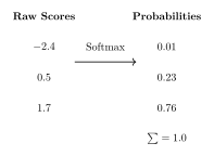
Because of the exponential in the Softmax formula, even small differences in raw outputs correspond to meaningful separation within probabilities—which is exactly the behavior we want.
5.3 Recurrent Neural Networks (RNNs)
While convolutional neural networks represented a breakthrough in generative modeling, they struggled with contextualizing long-range relationships between data during the generation process.
Recurrent Neural Networks offer the first steps at a solution, and are architectures that maintain an internal state which keeps track of sequential inputs. Mathematically, an RNN can be described by:
Where is the current hidden state, is the previous hidden state, is the current input, and are weight matrices, and is a bias term.
The main challenge these models face is maintaining cohesive context when generating large amounts of text. As such, they can be repetitive and, worse yet, spiral into nonsensical ideas. This phenomenon is dubbed the vanishing gradient problem (since it stems from gradients shrinking over long backpropagation), and has proved a serious limitation for tasks like text generation, where generating cogent narratives and solving problems logically can be challenging.
5.3.1 LSTM
Enter Long Short-Term Memory (LSTM) networks, a type of recurrent neural network that retains long term information through a series of "gates", which are themselves neural networks that learn what previous information to discard vs. what to keep.
Each LSTM cell maintains two internal states that function as the network’s ’memory’: the long-term cell state and the current hidden state, which together inform future outputs. These memory-like states allow LSTMs to learn dependencies over hundreds of time steps, since they provide direct pathways for gradients to flow—essentially for the model to update—through time via the cell state.
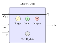
The LSTM above uses both cell state () and hidden state () with three gates: forget (), input (), and output (). This architecture creates pathways for long-term information flow.
5.3.2 GRU
Gated Recurrent Units (GRUs) were introduced as a further enhancement to LSTMs, and introduced a more computationally efficient approach to achieve similar results. With shorter sequences, GRUs perform nearly identically to LSTMs.
Rather than maintaining separate cell and hidden states, GRUs use a single hidden state and just two gates: a reset gate and an update gate.
The update gate determines how much of the previous state to retain, while the reset gate controls how much of the previous state to use in computing the new candidate state. In this way, the update gate combines the functionality of an LSTM’s forget and input gates.
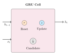
The GRU above simplifies the LSTM approach with only hidden state () and two gates: reset () and update (). This more compact design preserves pathways for long-term information flow.
5.4 Transformers
With the background of CNNs, LSTMs, and GRUs, the inception and rise of the Transformer architecture feels more like a natural progression than some magical breakthrough out of left field.
While each of these sequential architectures represented a great leap in long range contextualization, LSTMs and GRUs still struggle when dealing with properly utilizing prior information, either for logical deduction or meaningful cohesion across lengthier stories.
In 2017, a team of Google researchers released the paper "Attention is All You Need", which outlined an “attention” mechanism for capturing long-term context, and their proposed architecture, dubbed the “Transformer”. Transformers have since become the foundation of many recent advances in AI, powering large language models and image diffusion models.
5.4.1 Attention Mechanism
Fundamentally, attention allows a model to focus on relevant parts of its input when generating each part of its output.
Recall that LSTMs must pass information sequentially through states. Attention, on the other hand, creates direct connections between all token positions. When generating each word, the model can thus directly "attend" to any previous word, weighing their relative importance.
Put more simply, rather than “deciding” which sections of the previous output to look at, a Transformer is always looking at all previous parts of the output, and dynamically assigning “attention scores” to each token or word to indicate how important that segment is. This proved an enormous leap forward for generating meaningful language.
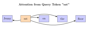
The above diagram illustrates the attention mechanism in Transformers: here, the query token "sat" (orange) interacts with its keys (the other tokens in blue).
For an example of Attention at work, consider the following sentences: "After studying the new drug’s effects on mice, the scientists found promising results. However, they need more testing."
Here, the transformer must understand that "they" refers to the drugs (not the mice or scientists) and that "testing" refers to drug trials (not academic exams). It does this by allowing "they" and "testing" to attend to relevant earlier context like "scientists" and "drug’s effects," building a coherent understanding of the narrative.
5.4.2 Self-Attention
For each individual token, a transformer computes three vectors: a query (what it’s looking for), key (what it matches against), and value (information it carries). These vectors essentially encode information about the role of that token in the sentence, and are used to calculate the aforementioned “attention scores” that dictate how much emphasis is placed on surrounding pieces of context.
For each position, the dot product of its query vector with all positions’ key vectors produces attention scores. After softmax normalization, these scores weight the value vectors to produce the final attended representation. These dot products represent compatibility scores—i.e how relevant each context token is to the current token being processed. The formula for this operation is:
where we divide by to normalize the size of the dot products (and prevent them from exploding).
An important note: there is nothing incredibly special about the way these three vectors are initialized. The real breakthrough in this approach lies in the fact that over time, these vectors start to encode meaningful information (as the model is trained), and because they represent the entire sequence length, they can meaningfully encode these long-range dependencies.
Again, this is best conceptualized through an example. Consider the sentence "The mouse wanted the cookie because it was hungry." When processing "it", self-attention helps determine the referent by computing attention scores with previous words. The model might assign high attention weights to "mouse" and "hungry," understanding that the mouse, not the cookie, was the hungry one.
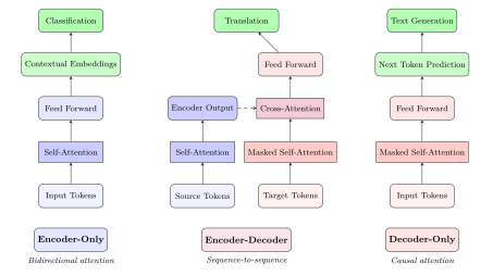
Transformers use two primary attention patterns. Bidirectional attention lets each token attend to all other tokens in the sequence, allowing for rich, complete contextualization.
Causal or masked attention restricts each token to only attend to previous tokens in the sequence. This prevents the model from peeking ahead at the future tokens it is trying to predict.
These patterns are typically used in different transformer architectures: bidirectional attention in encoder models focused on understanding (like BERT), and causal attention in decoder models designed for generation (like GPT), with encoder-decoder models using both patterns. More on these in the following section.
5.4.3 Transformer Architectures
There are three primary forms of transformer models.
Encoder-only models use the aforementioned bidirectional attention to build representations of input text. As such, they are strong at tasks like classification that benefit from looking at all the context collectively.
Decoder-only models, on the other hand, use causal attention to generate text autoregressively. They thus excel at generation tasks.
A third architecture, Encoder-decoder, combines both components, and is strong for tasks that require transforming one sequence of data into another one—such as translation.
5.4.4 Multi-head Attention
Multi-head attention allows transformers to run multiple self-attention operations in parallel, each with its own learned query, key, and value matrices. This allows the model to capture different types of relationships simultaneously. The formula extends our previous self-attention: where
In practice, each attention head learns different relationships within the data, which is why assembling them in a single model is extraordinarily powerful. In text generation, one attention head may learn temporal relationships, while another captures grammatical relations, and a third understands possession.
Transformers are powerful, but they can be VERY computationally expensive. Since every token attends to every other token, transformers scale quadratically.
5.4.5 Modern Transformer Optimizations and Variants
To alleviate the quadratic computational complexity that comes with full attention architectures, linear attention transformer variants approximate attention in time.
One method for this is KV caching. This builds off a pretty neat realization: that previously generated tokens’ key and value vectors remain constant when generating new tokens. By caching these values—rather than recalculating them with every additional token—models achieve linear time complexity with long sequence lengths.
Transformers can also be extended to image inputs through Vision Transformers, which tokenize patches of images and run attention on them. Compared to earlier vision models, vision transformers are strong at capturing hierarchical relationships, which is critical to contextualizing an entire scene.
There are also Mixture of Experts models, which build specialized "experts" that route tokens to different mini models based on the token’s content. Improving these variants is an active research area.
Together, these architectures represent a meaningful way in which ML systems have been improved over time for specific tasks. From the basic perceptron to the techniques powering Large Language Models such as ChatGPT, neural network architectures are a major way that we address computational constraints.
6 Training & Evaluation
Training and evaluation are components of a feedback loop through which ML models learn from data and demonstrate their effectiveness. These processes rely on error functions to guide parameter optimization, alongside metrics to objectively measure model performance.
While the mechanics of machine learning are somewhat different from those of biological learning, the core idea is fundamentally the same. Given thousands (or millions) of observations, learning involves finding underlying patterns and understanding which behavior is advantageous—and which is not. This is a process we refer to as training in machine learning.
Mathematically, this is formalized through error (or loss) functions, a major topic in this chapter. Once a model is trained, there are several ways to evaluate effectiveness, which we also discuss.
6.1 Data Preprocessing
Raw data requires significant preparation before model training. Data preprocessing transforms raw data into a format suitable for ML algorithms. This entails handling missing values, (either by extrapolating or ignoring them), as well as scaling different modalities of data to prevent overemphasizing certain features.
For example, if some class of data is underrepresented in a training set, you can increase the number of samples you draw from that class during the training process. One way to accomplish this is the Synthetic Minority Over-sampling Technique (SMOTE), which upscales data with a minimized risk of overfitting.
Best practice is to use the most "high-quality" data from our training set, which generally involves removing noisy samples and corrupted entries. This can be done at scale with automated quality scoring techniques.
Another issue is deduplication. At a small scale, this can be trivial, but with larger datasets, it quickly grows computationally infeasible. Several techniques such as locality-sensitive hashing, embedding-based similarity detection, and distributed processing frameworks have been developed to address this, but it remains a challenge. Especially important is ensuring there is no data leakage—or shared entries—between the training set and the test set.
You can also choose how to handle outliers in a dataset, as well as how to encode the data (as mentioned before with embedding models). In some cases, large models can compensate for poor choices in the data processing pipeline (i.e., a model can learn to ignore outliers), but typically these decisions dictate much of the later development process: from cost to time to output quality.
Finally, human annotation collection yields labeled data in otherwise unsupervised learning contexts. Checking that these annotations are correct typically involves building robust and consistent instruction frameworks for those labeling the data.
Even a small amount of mislabeled data can be crippling for frontier models, since the quality of the dataset helps dictate the upper bound for how well a model can perform.
6.2 Model Compression
Model compression techniques reduce model size and computational requirements while maintaining performance.
One relatively straightforward way to do this is through Quantization, which involves reducing the numerical precision with which you store weight and activation values.
For example, reducing the standard representation of 32 bit floating-point numbers down to less precise 8 bit data types can dramatically improve model training and inference speed, since the hardware bottlenecks are eased. This approach has been extraordinarily successful, often only minimally reducing performance.
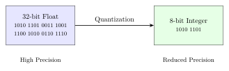
In the above diagram, a 32-bit floating point representation is reduced to an 8-bit integer representation to achieve lower memory usage and faster computation.
Quantization focuses on reduced precision for inference; mixed precision training, on the other hand, leverages lower precision formats during the training process itself. These formats include BF16 (Brain Floating Point) and FP8 formats, which use fewer bits than standard FP32. These techniques reduce memory bottlenecks, but also increase risks for numerical stability (critical for model convergence). Regardless, they are widely used as training modern ML models approaches the limitations of our current hardware.
Another technique here is pruning, where you systematically remove redundant or less important parameters from a network, which prevents us from ending up with an over-parametrized model. Finally, engineers can also implement knowledge distillation, which involves training a small, lightweight model to mimic behavior of a larger one. Similarly, weight matrices can be broken down into their most important low-dimensional components through Low-rank factorization.
6.3 Error Functions
In ML, the terms "loss" and "error" are often used interchangeably.
A loss function quantifies how poorly a model performs by measuring the difference between a model’s predicted outputs and actual desired values for individual data points. The error function (or cost function) typically refers to the aggregate loss across the entire dataset, usually calculated as the average of all individual loss values. These are important for both training (by providing gradients for optimization) and evaluation (by measuring model performance).
Loss/error functions differ depending on the problem type, primarily falling into two categories: classification functions (for predicting probabilities for classes or labels of data) and regression functions (for predicting continuous numeric values).
6.3.1 Regression Tasks
Mean Squared Error (MSE): MSE calculates the average of squared differences between predicted and actual values. Its smooth quadratic (U-shaped) curve means it provides stable gradients during optimization and penalizes large errors much more heavily than small ones.
We often use MSE when outlier detection is important or when large errors are particularly undesirable, and when working with data where the scale of errors matters.
Mean Absolute Error (MAE): MAE measures the average absolute difference between predicted and actual values.
MAE has a V-shaped linear curve which treats all error magnitudes proportionally—a mistake twice as large receives double the penalty. Thus, MAE is more robust to outliers compared to MSE, and we can use it when we want a model to be less sensitive to occasional large errors.
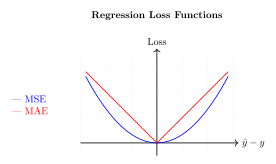
In the above graph visualization, MSE (Mean Squared Error) penalizes large errors more heavily than MAE (Mean Absolute Error).
6.3.2 Classification Tasks
Binary Cross-Entropy: BCE measures the performance of a classification model whose output is a probability value between 0 and 1. The logarithmic curves approach infinity at the extremes, so when a model is completely confident but wrong, the penalty is extremely severe. For positive examples (y=1), BCE penalizes low probability predictions; for negative examples (y=0), it penalizes high probability predictions.
Hinge Loss: Hinge loss has a flat region (zero loss) for confident correct predictions and a linear penalty for incorrect or insufficiently confident predictions. This creates a "margin" around the decision boundary, allowing the model to find a classification boundary with maximum separation between classes.
Unlike BCE, hinge loss doesn’t penalize correct predictions beyond any threshold—it only cares about mistakes. So we often use it for classifiers like Support Vector Machines, or when you need a clear wide decision boundary between classes.
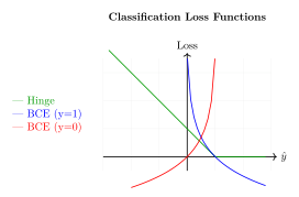
In the above graph visualization, Hinge loss creates a margin while Binary Cross Entropy (BCE) shows behavior for positive (blue) and negative (red) classes.
6.4 Evaluation Metrics
6.4.1 Regression Metrics
The following metrics quantify prediction errors in regression tasks:
Root Mean Squared Error (RMSE): RMSE calculates the square root of the average squared differences between predicted and actual values (or in other words, the square root of MSE). This allows RMSE to return error measurements in the same units as the original data. Like MSE, RMSE is sensitive to outliers due to the squared term, penalizing large errors disproportionately. We typically use RMSE when reporting errors in the original scale of the data is important, and when larger errors should receive more weight in the evaluation.
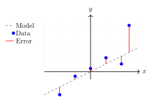
Mean Absolute Percentage Error (MAPE): MAPE gives prediction accuracy as an average percentage error, making it scale-independent. By calculating the absolute percentage difference between actual and predicted values, MAPE allows for comparison across different datasets with varying scales.
Still, MAPE has some limitations—it’s undefined for actual values of zero and can give misleading results for small actual values. We use MAPE when relative errors are more important than absolute ones, and when comparing model performance across different scales or units.
R-squared (): measures the proportion of variance in the dependent variable that’s explained by the model. It compares the fitted model to a simple baseline that predicts the mean of the data.
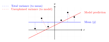
In the preceding figure, the blue dashed lines show total variance (distances from data points to the mean), while red dashed lines reflect unexplained variance (distances to model prediction). .
The value of ranges from 0 to 1 (or negative in the case of poor fit), with higher values describing better fit. A value of 0.7 means the model explains 70% of the variance in the data. We use for a standardized measure of fit comparable across different dependent variables, and to see how our model performs compared to simply predicting the mean.
Adjusted R-squared: Adjusted modifies the standard to account for the number of "predictors" in the model. It penalizes additional predictors that don’t add significant explanatory power, which resolves an issue where normal increases (or stays the same) when more predictors are added.
This makes it useful for comparing models with different numbers of features. We can use this when performing feature selection, as if adding a predictor causes Adjusted to decrease, that predictor likely isn’t improving the model in a meaningful way.
6.4.2 Classification Metrics
For classification tasks, we can evaluate different aspects of model performance:
Accuracy: Accuracy measures the proportion of correct predictions among all predictions made. It is a simple metric that works for balanced datasets where all classes appear a similar number of times.
However, accuracy can be misleading with imbalanced datasets—a model predicting the majority class for all inputs will have high accuracy but fail resoundingly on the minority class. For example, in a medical diagnosis setting with 95% healthy patients, a model that predicts "healthy" for all patients will technically achieve 95% accuracy.
Precision and Recall:
Precision measures how many of the predicted positive instances are actually positive. Put simply, when the model returns "yes," how often is that correct? High precision minimizes false positives, significant when false alarms are undesirable (e.g. spam detection, marking an important email as spam has consequences).
Recall (also referred to as sensitivity) measures how many of the actual positive instances the model correctly identified—when the answer is "yes", how often does the model return that? High recall minimizes false negatives, most important when missing positive cases is dangerous (e.g., cancer screening). These metrics together describe different aspects of model performance that accuracy alone could conceal.
F1 Score:
F1 score is the harmonic mean of precision and recall, and gives a single metric balancing both. The harmonic mean penalizes extreme values more than the arithmetic mean, meaning a model must perform well on precision AND recall to achieve a high F1 score. This means F1 is valuable for imbalanced datasets (addressing the problem we earlier noted with accuracy).
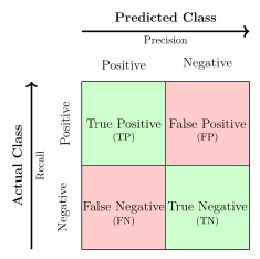
In the confusion matrix above, green cells represent correct predictions, while red cells represent errors. Precision is the reliability of positive predictions (rows), recall is the ability to find all positive cases (columns).
The Receiver Operating Characteristic (ROC) Curve plots True Positive Rate (TPR) against False Positive Rate (FPR) across classification thresholds, helping to visualize the tradeoff between sensitivity and specificity. A perfect classifier’s curve goes straight up and to the right.
The Area Under Curve (AUC) measures overall performance: 1 is perfect classification, while 0.5 suggests randomness. AUC is threshold-invariant and works well with imbalanced datasets by considering each class independently. Mathematically, the area under the curve represents the probability that a model will rank a random positive example higher than a random negative one.
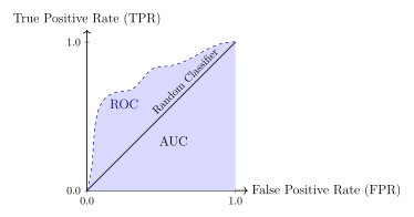
In the ROC curve above, you can see True Positive Rate vs False Positive Rate across thresholds, where the diagonal represents random classification. The AUC (area under curve) quantifies classifier performance, with values closer to 1 indicating better performance.
6.5 Training Techniques
6.5.1 Optimization Algorithms
Optimization algorithms are the processes by which, through training and fine-tuning, models reach convergence (the point where further iterations do not significantly change parameters).
Stochastic Gradient Descent (SGD), previously discussed, is one of the most widely-used optimization methods, continuously updating the weights and parameters through minimizing loss by moving in the direction of the gradient.
The update rule for SGD is the following: , where is the learning rate. This updates model parameters in the opposite direction of the gradient to minimize error.
The Adaptive Moment Estimation (Adam) optimizer incorporates ideas such as momentum (adding inertia to the optimization process) and adaptive processes (resistance to the optimization process). It utilizes the exponentially weighted average of the gradients to accelerate convergence.
This all comes at a compute cost; Adam requires two separate rolling statistics (first and second moments) for each parameter in the model, which scales up with large models—especially ones using 16 bit precision (more on this in section 6).
Adam combines the benefits of two other extensions of SGD: AdaGrad, which maintains per-parameter learning rates, and RMSProp, which adapts these rates based on recent gradients. Adam computes both first-moment (mean) and second-moment (uncentered variance) estimates of the gradients:
(First moment). This calculates a weighted moving average of gradients to add momentum to the optimization direction.
(Second moment). This is the exponentially weighted moving average of squared gradients, capturing the variance, to adapt learning rates for each parameter.
These moments are bias-corrected (meaning they are adjusted to account for initial zero-value initialization effects on parameter estimates), then used to update parameters:
Here, and are decay rates often set to 0.9 and 0.999 respectively, and is a small constant for numerical stability. It updates parameters using the normalized gradient direction with adaptive step sizes.
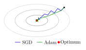
The following diagram visually compares the paths of SGD vs Adam on a loss surface, showing how Adam’s adaptive learning rate helps it navigate more efficiently toward the optimum.
In the following graph, we visualize the convergence patterns of these optimization algorithms; SGD (blue) steadily decreases the loss but converges more slowly, while Adam (green) achieves faster convergence with potential minor oscillations near the optimum.
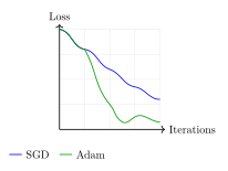
In practice, Adam has a few advantages. It is resilient to noisy gradients, it can navigate around saddle points (non-maxima where the gradient is zero), and it supports automatically adjusting learning rates per parameter. Still, SGD often generalizes better, due to its noisier updates providing built-in regularization. The choice of optimizer depends on the scenario.
6.5.2 Batch Normalization
It is common practice to normalize data (to zero mean and unit variance) before inputting it to a model. Different features could have vastly different scales/ranges of values. In order to compare across features, you independently find the mean and variance for each feature and then, for each feature value, subtract the mean and divide by the standard deviation. This results in all feature values across features being on the same scale and centered around 0. Normalization speeds up convergence by making the loss landscape more even.
Batch normalization extends this concept to hidden layers in deep networks. Essentially, after each hidden layer, you have the same problem where the outputs of one layer are no longer normalized. So, we must normalize again after each activation—this is where batch normalization comes in. During training, normalization is computed with respect to the current mini-batch of data (hence "batch" normalization), requiring many examples to be processed simultaneously to calculate meaningful statistics.

Unlike the input layer, batch normalization doesn’t have to be normalized around 0. It can be shifted (to a different mean) and scaled (to a different variance), by multiplying the normalization values by a factor gamma and adding a factor beta . This is expressed mathematically as:
where and are batch statistics ( is mini-batch mean and represents mini-batch variance).
This technique speeds up training by stabilizing the distribution of layer inputs and reducing internal covariate shift. During inference or test time, batch norm layers use the empirical values which are running averages of the mean and variance accumulated during training, ensuring consistent normalization.
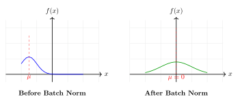
In the above graphs, we can see the impact of Batch Normalization on activation distributions. Before batch norm, in the first figure, the distribution is skewed with arbitrary mean. After batch norm, in the second figure, BN standardizes the distribution to zero mean, making network training more stable.
Batch Normalization has historically been useful for training CNNs. With more modern architectures (like Transformers), a similar technique called Layer Normalization is often implemented. Layer Norm normalizes across the feature dimension for each individual example, which allows for variable sized batches. Batch sizes typically differ between training and testing, a discrepancy normalizing by layer helps alleviate.
RMSNorm simplifies this further by normalizing only on the root mean square of activations (skipping the mean centering step). This incrementally improves compute scaling with model size.
6.5.3 Dropout
Dropout prevents overfitting by randomly deactivating neurons during training with probability (typically 0.5). Each training sample uses a different dropout pattern, while inference uses all neurons with outputs scaled by . This approach has a few benefits; it forces redundant feature learning, prevents neuron co-adaptation, and approximates ensemble learning within a single network. Mathematically, for each neuron with output , dropout applies:
Where is a scaling factor, typically , that maintains expected output magnitudes.
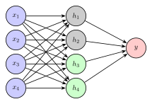
The above diagram illustrates how with Dropout, during training, hidden nodes and may be randomly excluded from backpropagation. During inference, all neurons are active as an ensemble of multiple "thinned" networks.
Dropout’s ensemble impact comes from an exponential number of "thinned" networks (around where is the number of neurons) sharing weights during training, collectively creating a regularization effect.
6.5.4 Learning Rate Scheduling
The learning rate is a hyperparameter that determines how large of steps to take when updating weights during optimization. Very low learning rates lead to slow model convergence, while high learning rates can lead to overshooting optima and divergent behavior. That said, it is difficult to properly select an appropriate learning rate from the start, and is often suboptimal to use the same learning rate throughout the entire training process.
Learning rate scheduling addresses this by dynamically modifying the learning rate through the course of the training process. Generally, schedules favor larger learning rates in earlier parts of training (where the parameters are still far from an optimum), and shrinking learning rates as training progresses (which allows better convergence).
The most straightforward way to implement this is through step decay, where the learning rate is reduced by some factor at given (not necessarily constant) intervals. Alternatively, this decay can be exponential or trigonometric for a smoother, and perhaps more rapid decrease. Many modern ML implementations also integrate "warm-up", which involves gradually increasing the learning rate at the start of training before applying other scheduling strategies.
Intuitively, this allows for our model to learn faster as it initially progresses towards an optimum, before transitioning to smaller, more subtle changes to prevent overshooting. It is a tradeoff between convergence speed and precision. In the first phase, larger learning rates allow the model to look at bigger swaths of our training landscape. The later phase with lower learning rates then focuses on small adjustments once a promising optima region is found.
6.5.5 Overcoming Hardware Bottlenecks
Addressing the memory bottleneck presented by hardware is a huge research area in AI development. Solutions include both system-level software and architectural optimizations.
At the lowest level, we have custom kernels, which are specialized pieces of GPU code that optimize hardware efficiency. There is also kernel fusion, which combines multiple sequential operations into a single kernel, eliminating memory overhead and extraneous operations. They are particularly helpful for operations like layer normalization and attention mechanisms in modern architectures—like transformers.
At the architectural levels, we have gradient accumulation— which as the name implies—accumulates gradients across several model passes (forward and backward) prior to updating model weights. This helps with memory bottlenecks.
Gradient checkpointing is another method to trade computation for memory. It involves ignoring several intermediate activations during a forward pass, and instead computing them during backpropagation.
Gradient clipping refers to limiting the maximum size of gradients (which typically grow over time). This combats the "exploding gradient problem", which hurts model convergence and numerical stability.
Finally, models can be trained across disparate hadware using distributed training approaches. Fully Sharded Data Parallelism (FSDP) and ZeRO allow for sharing parameters, gradients, and optimizer states across devices, and only regathering full parameters when needed (during forward and backward passes). This parameter splitting can also be done through tensor parallelism, which divides high dimensional matrices across hardware. Decentralized training has been particularly effective as hyperscalers (players training large AI models) look to expand their capabilities.
6.5.6 Curriculum Learning
Curriculum learning is another method to optimize the training process. It involves gradually increasing the "difficulty" of training examples (as opposed to training in an arbitrary order), which can lead to quicker convergence and more optimal learning.
6.5.7 Fine Tuning
While conceptually very similar to transfer learning, fine-tuning is the process of taking a pre-trained model and adapting it to a specific task by continuing training on a new, usually smaller, dataset (typically 1 to 10 percent the size of our pre-training dataset). This is essentially specializing your model to a specific use-case, and is incredibly powerful, especially when training data is extremely limited.
There are several ways this can be implemented. The more involved version, "full" fine-tuning involves updating all model parameters during the additional training process. "Partial" fine-tuning, on the other hand, leaves most early layers frozen (weights don’t get updated) and updates only a couple of final layers. Fine-tuning typically employs a small learning rate, so as to not radically change existing parameters from the pre-trained model.
6.5.8 Transfer Learning
Training ML models is expensive in terms of time, compute, and funding. As researchers experimented with new applications, they found that they could take models that had been applied to different problems and use them as a starting point for tackling a new problem. This approach, called transfer learning, leverages the fact that models often learn generalizable features in their early layers. For instance, a vision model might learn to detect edges, shapes, and textures that are useful across many visual tasks, as would a language model already trained on a massive, general corpus of text data.
7 Advanced Topics
Building on the foundations we’ve established in earlier sections, the following topics reflect specialized applications and emerging paradigms. While we will barely scratch the surface of these areas, when you come across any of these topics in the future, you will have seen it before.
To start, we’ll review basics of graph theory and examine graph neural networks.
7.1 Graphs and Graph Theory
Graphs provide a framework for modeling relationships through nodes and edges. A graph consists of a set of nodes, called vertices , and a set of links/connections, called edges .
7.1.1 Basic Graph Properties
Direction: Edges can be directed (one-way) or undirected.
Weight: Edges can carry weights (distances, costs).
Degree: Number of edges connected to a vertex.
Walk: Sequence of alternating vertices and edges where each edge connects its adjacent vertices.
Path: Walk with no repeated vertices.
Connected: A graph where there exists a path between any two vertices.
Cycle: Path returning to starting vertex.
Example: Graphs
For graph with vertices :
Ordered pairs (directed edges):
Unordered pairs (undirected edges):
With weights:
When representing graphs computationally, we often use adjacency lists or adjacency matrices. This transformation encodes the graph structure into a linked list or matrix structure where each entry indicates connection strength between nodes.
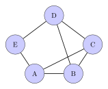
For an unweighted graph, the adjacency matrix is defined as:
For weighted graphs, the binary values are replaced with edge weights. Several traversal strategies exist: Breadth-First Search (BFS) explores level by level, while Depth-First Search (DFS) explores as far as possible along each branch before backtracking. While originally developed for trees, these algorithms also work on general graphs by tracking visited nodes.
Sample Graph Traversal Process:
1. Start at designated root node
2. Mark current node as visited
3. Explore neighboring nodes
BFS: Visit ALL neighbors before moving to next level
DFS: Visit ONE neighbor and its children completely before trying siblings
4. Repeat until all nodes visited
7.1.2 Special Graph Structures:
Many graphs have properties that resemble "special" graph structures. These include trees (connected graphs with no cycles), directed acyclic graphs (DAGs, directed graphs with no cycles), complete graphs (where every vertex connects to every other vertex), and bipartite graphs (where vertices divide into two sets with edges only between sets, not within).
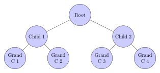
Modern approaches transform these discrete graph structures into continuous vector spaces while preserving their underlying relationships. By taking random walks through graphs, you can generate sequences of connected nodes that help algorithms learn meaningful embeddings. This forms the foundation for powerful techniques like node2vec and DeepWalk, which create vector representations that capture the graph’s structure.
Several specialized graph structures appear frequently in machine learning. Trees provide a cycle-free structure perfect for decision-making algorithms. Directed Acyclic Graphs allow multiple paths forward without loops, making them ideal for representing neural network computations. Bipartite graphs (bipartite means two parts) with two distinct sets of nodes model multi-object interactions. Graph theory offers various algorithms for exploring and analyzing these structures, including traversal and dimensionality-reduction techniques.
7.1.3 Graph Neural Networks
Graph Neural Networks (GNNs) process data structured as graphs, capturing relationships between entities. They operate through message passing between nodes, aggregating neighbor information to update representations. This architecture suits tasks from molecular property prediction to social network analysis.
Message Passing Framework:
Where U is UPDATE and A is AGGREGATE.
Key challenges include handling variable graph sizes, preventing over-smoothing of node features, and scaling to large graphs. Recent advances focus on improved architectures and efficient training methods.
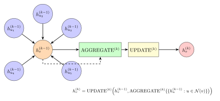
7.2 Time Series Analysis
Time series analysis addresses prediction tasks with temporal components, like stock prices. Autoregressive (AR) models predict future values based on past data. An AR(1) model considers the immediately preceding value, while AR(n) examines previous points, offering improved accuracy at higher computational cost.
Moving average (MA) models learn from past prediction errors rather than values. An MA(1) model adjusts based on its previous error, while MA(n) incorporates n past errors. ARIMA models combine both approaches, incorporating previous values and errors while examining higher-order differences between data points. For data with recurring patterns, Seasonal ARIMA models leverage repeating patterns..
7.3 Diffusion Models
Diffusion models represent a novel approach to generative AI through iterative noise manipulation. The process involves gradually adding noise to data during training, then learning to reverse this process for generation. Unlike GANs, diffusion models offer more stable training and better quality control.
Diffusion Process:
These models excel in text-to-image generation, image editing, and other creative applications.
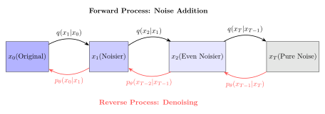
7.4 Agentic AI
Agentic AI refers to AI systems that make autonomous decisions to achieve complex goals, typically without constant supervision. Multi-step reasoning enables agentic AI to use language models to break down complex problems into sequential tasks, track context across steps, and adjust dynamically based on new data.
By employing planning graphs, decision trees, and pathfinding algorithms, these systems refine decision-making through iterative analysis and structured reasoning. Multi-agent systems enable collaboration across multiple agents to coordinate actions and share information.
Such systems can coordinate through centralized or decentralized networks, using hierarchical or flexible structures to manage collaboration, while coalition and team-based coordination enable dynamic reorganization in complex environments.
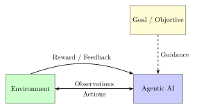
8 Conclusion
This primer has hopefully served as a brief introduction to foundational machine learning concepts and practices. While we attempt to be somewhat comprehensive, this document still represents only a snapshot of a rapidly evolving field. We strongly encourage you to explore these topics further through the provided resources and stay engaged with emerging developments.
Further Mathematical Foundations
The following are a few topics out of scope for this primer, but that you may find valuable in your readings:
Singular Value Decomposition
By the same mechanisms that let us multiply matrices, you can also break them into products of other matrices. SVD decomposes any matrix into three components:
SVD Decomposition
, where:
: left singular vectors (m × m)
: diagonal matrix of singular values (m × n)
: transposed right singular vectors (n × n)
U and V contain "directions" in the input and output space, and contains scaling factors (like eigenvalues but always non-negative). Together, they describe how the matrix transforms data; singular values and their vectors are the building blocks of linear transformations. By breaking down matrices this way, SVD helps approximate, compress, and understand complex data by keeping only the most important components. That is, you maintain the structure of our data while removing some complexity.
Hypothesis Testing
Statistical hypothesis testing is a framework for uncertainty-based decisions by specifying hypotheses, choosing a significance level, and calculating a test statistic. The null hypothesis represents the status quo, while the alternative hypothesis is the claim of interest.
For instance, when evaluating a model, your null hypothesis might be "this model performs no better than random chance", while an alternative hypothesis could be "this model outperforms random chance".
The p-value is the probability of observing our data (or more extreme data) if the null hypothesis were true. It is NOT the probability that a hypothesis is correct. When you claim a model achieves "statistically significant" improvements, you are actually saying the probability of seeing such improvements by chance, assuming the null hypothesis is true, is very small (typically less than 5%).
Type I errors (false positives) occur when you reject a true null hypothesis, while Type II errors (false negatives) happen when you fail to reject a false null hypothesis. Minimizing improves precision (the ratio of true positives to all predicted positives) and minimizing improves recall ((the ratio of true positives to all actual positives) in machine learning evaluations. More on this in section 6.
Type I and type II errors are commonplace. It is important to keep in mind which you should be optimizing for as different scenarios have different consequences.
Maximum Likelihood Estimation (MLE)
MLE finds the parameters most likely to reproduce some observed data. In neural networks, "minimizing loss" means maximizing the likelihood of training data.
MLE Process
1. Express the probability of observations given parameters
2. Find the parameters maximizing this probability
3. Often log-likelihood is used for computational ease:
For Gaussian distributions, MLE gives sample mean and variance as optimal parameters. Modern architectures extend this principle to complex parameter spaces. Mathematically, MLE seeks the parameter estimate that maximizes the likelihood function of the parameters given the observed data. This function is calculated as the product of the probability of each individual data point given those parameters.
Common loss functions directly correspond to negative log-likelihoods: mean squared error assumes Gaussian noise, while cross-entropy loss corresponds to categorical distributions.
Further Reading
Below we’ve compiled (in no particular order) some resources to help you go deeper on many of the concepts the Grimoire has discussed, as well as consider some more advanced topics.
In particular, we’d love to highlight the incredible content that Grant Sanderson, Andrew Ng, and Andrej Karpathy have shared and made freely available, linked below. This is by no means an exhaustive list—think of it as simply a starting point for further exploration.
Textbooks & Courses
Deep Learning (Goodfellow et al.)
Speech & Language Processing (Jurafsky)
Probabilistic Machine Learning (Murphy)
Information Theory, Inference, and Learning Algorithms (MacKay)
Interpretable Machine Learning (Molnar)
Deep Learning Specialization (Andrew Ng)
Articles
The Illustrated Transformer (Jay Alammar)
Attention? Attention! (Lilian Weng)
A Recipe for Training Neural Networks (Karpathy)
A Deep Dive into GANs (Lilian Weng)
Feature Visualization (Olah et al.)
YouTube Channels & Videos
Research Papers and References
Vaswani, A. et al. Attention Is All You Need. arXiv:1706.03762, 2017.
He, K. et al. Deep Residual Learning for Image Recognition. arXiv:1512.03385, 2016.
Devlin, J. et al. BERT: Pre-training of Deep Bidirectional Transformers. arXiv:1810.04805, 2018.
Kipf, T. N. & Welling, M. Semi-Supervised Classification with GCNs. arXiv:1609.02907, 2016.
Krizhevsky, A. et al. ImageNet Classification with Deep CNNs. NeurIPS, 2012.
Bahdanau, D. et al. Neural Machine Translation by Jointly Learning to Align and Translate. arXiv:1409.0473, 2014.
The Annotated Transformer. Harvard NLP.
Karpathy, A. The Unreasonable Effectiveness of RNNs. 2015.
Olah, C. Understanding LSTM Networks. 2015.
Zaremba, W. et al. RNN Regularization. arXiv:1409.2329, 2014.
Hinton, G. & van Camp, D. Keeping Neural Networks Simple. COLT, 1993.
Vinyals, O. et al. Pointer Networks. arXiv:1506.03134, 2015.
Vinyals, O. et al. Order Matters: Sequence to Sequence for Sets. arXiv:1511.06391, 2015.
Huang, Y. et al. GPipe: Pipeline Parallelism. arXiv:1811.06965, 2018.
Yu, F. & Koltun, V. Multi-Scale Context Aggregation. arXiv:1511.07122, 2015.
Gilmer, J. et al. Neural Message Passing. arXiv:1704.01212, 2017.
Santoro, A. et al. Neural Network for Relational Reasoning. arXiv:1706.01427, 2017.
Chen, X. et al. Variational Lossy Autoencoder. arXiv:1611.02731, 2016.
Majumdar, A. Deep Learning History. GitHub, 2023.
Bishop, C.M. Pattern Recognition and Machine Learning. Springer, 2006.
Murphy, K.P. Probabilistic Machine Learning. MIT Press, 2022.
Karpathy, A. A Recipe for Training Neural Networks. Blog, 2019.
Yang, L. et al. Diffusion Models: A Comprehensive Survey. arXiv:2209.00796, 2022.
Gao, J. et al. Retrieval-Augmented Generation: A Survey. arXiv:2312.10997, 2023.